General scheme of process of identification
Plan:
• main stages of identification;
• aprioristic and a posteriori information;
• criteria and indicators of quality of identification.
• classification of methods of identification.
• principles structural and parametrical identification;
• printsiaa of active and passive identification.
Let's consider the list of approximate stages of identification. The technology of mathematical modeling of technical systems generally assumes accomplishment of the following main stages:
1. The formulation is more whole. At the heart of any task, a problem of modeling information on what dependences us lies interest what its purposes of its use. This information determines an object. These representations can be very approximate, but always reflect some of its properties sufficient for the effective formulation of the purposes of modeling. Usually in modeling tasks the objectives are achieved by maximization or minimization of some criterion set in the form of criterion function.
2. Studying of an object. At the same time it is required to understand the happening process, to determine object borders with the environment surrounding it if those are available. Besides, at this stage the list of all input and output parameters of an object of a research and their influence on modeling goal achievement are determined.
3. Descriptive modeling (development of conceptual model) - establishment and verbal fixing of the main communications of input and output parameters of an object.
4. Mathematical modeling (development of mathematical model) - the translation of descriptive model into formal mathematical language. The purpose registers in the form of function which usually call target. The behavior of an object is described by means of ratios, input and output parameters of an object at this stage depending on complexity of the researched problem can arise a number of tasks of net mathematical nature.
5. Choice (or creation) method of the solution of a task. At this stage for the arisen mathematical task the suitable method will be selected. In case of the choice of such method it will be necessary to pay attention to complexity of a method and the consumed computing resources. If the suitable method by the shown criteria doesn't appear, then it is required to develop a new method of the solution of a task.
6. Choice or writing computer programs. At this stage the suitable program realizing the chosen decision method is chosen. If such program is absent, then it is necessary to write such program.
7. The solution of a task on the computer. All necessary information for the solution of a task is entered into memory of the computer together with the program. With use of the suitable program handling of target information and receipt of results of the solution of tasks in a convenient form is made.
8. Check of adequacy of model (verification of model).
9. The analysis of the received decision. The analysis of the decision happen two types: formal (mathematical) when compliance of the received solution of the constructed mathematical model is checked (in case of discrepancy the program, basic data, operation of the COMPUTER, etc.) and substantial (economic, technological, etc. is checked) when compliance of the received decision to that object which was modelled is checked. As a result of such analysis changes or amendments then all considered process repeats can be made to model. The model is considered constructed and finished if it with a sufficient accuracy characterizes activities of an object for the chosen criterion. Only after that the model can be used when calculating.
Check of adequacy is stated above in the form of one of modeling stages.
Mathematical modeling of technical systems assumes application of the following methods:
1. analytical;
2. numerical;
3. statistical (imitating);
4. analytic-imitating.
The choice of a specific method of modeling depends on many factors, including from:
• is more whole than modeling;
• difficulties of the researched system;
• difficulties of the model determined by the chosen level of its disaggregation;
• requirements to the nomenclature of the researched characteristics;
• requirements to accuracy of the received results;
• requirements to a community of the received results;
• requirements to costs of time for modeling;
• requirements to material costs;
• availability of special technical means for carrying out modeling;
• qualifications of the specialist who is carrying out modeling, etc.
Results of the comparative analysis of methods of modeling made at the high-quality level are provided in tablitse10.1 (braces noted the best values of each indicator).
Table 10.1
Results of the comparative analysis of modeling methods receipt of the tasks solution results in a convenient form.
| modeling Method | Complexity of a method | Community of results | Accuracy of results | Time comsumption | Material costs | Syntesis tasks |
| Analytical | {+} | {++++} | + | {+} | {+} | {+} |
| Numerical | ++ | +++ | ++ | ++ | ++ | ++ |
| Imitating | +++ | + | {++++} | ++++ | ++++ | ++++ |
| Combined | ++++ | ++ | +++ | +++ | +++ | +++ |
Initial information is necessary for the solution of problems of mathematical modeling and identification. She is conditionally divided into two look - aprioristic and a posteriori information. (aprioristic information and posteriori information).
In case an object is considered as "a black box", then as a rule use only a posteriori information.
"Black box" — the term used in the exact sciences (in particular, system engineering, cybernetics, etc.) for designation of system which mechanism of work is very difficult, unknown or unimportant within this task. Such systems usually have certain "entrance" for input of information and "exit" for display of results of work. The condition of exits usually functionally depends on a condition of entrances.
Use of aprioristic information on a research object (if it is available) in many cases facilitates a solution of the problem of identification.
Criteria and indicators of quality of identification. Formation of criterion of the quality characterizing adequacy of model to a real object is one of the main stages of identification.
Quantitatively degree of adequacy of model and an object can be estimated by comparison of their output signals when giving identical entrance impacts on an object and its model. Such comparison preferable on the basis of the new information other than that set of data which was used in the course of identification of an object.
The block diagram of calculation of Estimate of an error of model of a static object is provided on the figure 10.1.
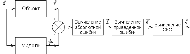 Figure 10.1. Block diagram of calculation of Estimate of an error of model
Let l of experiences at various levels of entrance influences  from area
  of their admissible values be carried out and realization of exits of an object
  and exits of model
  ,
,  is received.
Errors of model  and
and  for Estimate of her adequacy are calculated on formulas:

 ;
;
 ;
;

where  - the absolute, given and mean square errors of model on I to an exit ;
  - i value of an exit of an object and model in j experience
  ;
;  - the maximum change of i-go of an exit of an object at admissible values of entrances
 from area
  .
.
If size of these errors there is less some set positive number, then the model is adequate to an object.
Now we will consider Estimate of model of a dynamic object. Let's put that after identification the model of a one-dimensional object in the form of the linear differential equation of a look is received.
 (10.1)
where  - an entrance signal of model;
 - output signal of model;
n, m - the highest orders of derivatives;
and  respectively
  .
.
Let realization of an entrance  and an exit
  of an object on an interval of time
  , where
  - the realization length (observation time) be received. Now quality of model can be estimated by comparison and or directly on graphics (visually), or having entered some formal measure of distance between these signals.
Output signals of an object and model at the same entrance signal differ as their differential equations and initial states aren't identical. For Estimate of adequacy of model and an object we will enter criterion of their proximity on a difference of output signals, i.e. reactions to the same entrance signal , for example the following look:
 , (10.2)
where  - some convex function.
In particular:
 . (10.3)
Generally Estimate of adequacy is carried out for various forms of an entrance signal. From here the idea of need of averaging on entrance signals and entry conditions, i.e. entering of transaction of population mean of Estimate follows:
 . (10.4)
Expression of an output signal has quite difficult appearance that complicates an analytical research of dependence on model coefficients therefore also other criteria are entered. In particular, if the equation of model has an appearance
 (10.5)
that for Estimate of proximity of model and an object convenient appears functionality from the difference of entrance signals  of model and an object providing the same output signal:
 (10.6)
provided that  . In this case we will designate an output signal of model and an object.
Then, adding (10.5) in (10.6), we have
 (10.7)
i.e. the functionality in an explicit form depends on model coefficients that is convenient for an analytical research.
Developing this idea, it is possible to formalize convenient functionality for a general case of model (10.1)
 . (10.8)
Expression:
 (10.9)
is called the generalized model error. As function  , as a rule, accept a square of the generalized error
 . (10.11)
This functionality is convenient that it in an explicit form depends on parameters of model and on entrance and output signals of an object available to measurement. However in case of calculation of this functionality there are certain difficulties connected with differentiation of signals and , and also with need of accomplishment of transaction of population mean. The block diagram of calculation of the generalized error and Estimate of criterion I is provided on in the figure 10.2 where  - the operator of differentiation.
 Figure 10.2. The block diagram of calculation of the generalized error and Estimate of criterion I
However under the terms of physical feasibility it is possible to create only devices which order of numerator is less (or it is equal) than a denominator order, i.e. it is possible to realize devices with operators
 and
and  ,
,
where  - the polynomial of degree is more or equally
  ;
;  .
.
Then the block diagram of calculation of the generalized error  and Estimate of criterion
  will have an appearance, presented in the figure 10.3.
 Figure 10.3. The block diagram of calculation of the generalized error
 ; (10.12)
 . (10.13)
The scheme provided on on the figure 10.4 is equivalent to the block diagram represented in the figure 10.3.

Figure 10.4. The equivalent block diagram of calculation of the generalized error
Thus, the generalized error measured by means of physically implementable devices differs from the generalized error  in what is result of transformation by the filter with transfer function
  . Owing to an extremity of bandwidth of this filter there are misstatements of a signal of the generalized error. These misstatements will be that less, than more bandwidth of the filter.
If the size of errors of model and estimates of criteria of approach satisfy to quality requirements of model, then the model is considered adequate to an object and can be used for the solution of tasks of modeling, optimization and control. Otherwise the model needs to be enhanced by change of structure and introduction in it factors unaccounted earlier.
Дата добавления: 2017-05-02; просмотров: 1332;
Поиск по сайту
Узнать еще
- Asia. General characteristic.
- CARDIOVASCULAR SYSTEM SCHEME
- Cognitive processes
- Complex Antigens Are Degraded (Processed) and Displayed (Presented) with MHC Molecules on the Cell Surface
- Construction Processes
- European countries. General characteristic
- Factors influencing the process of translation.
- Fig. 2.5. Process of meiosis
Публикации по технике и механике
Публикации по биологии
Публикации по информатике
Публикации по строительству
Публикации по физике
Публикации по химии
Публикации по электронике

Публикации по искусству

Публикации по географии
Публикации по медицине